Related Content Outcomes:
- MA-S1 Probability and Discrete Probability Distributions
- S1.2: Discrete probability distributions
HSC, We Have A Problem
The HSC Syllabus does not give a clear definition of what a random variable actually is – it rather describes what it does:
know that a random variable describes some aspect in a population from which samples can be drawn
Mathematics Advanced Stage 6 Syllabus, p. 47
In the glossary, it says this:
A random variable is a variable whose possible values are outcomes of a statistical experiment or a random phenomenon.
Mathematics Advanced Stage 6 Syllabus, p. 73
which isn’t exactly clear when it’s used the word ‘variable’ twice in the sentence. My favourite part about this is that even though it is called a random variable, it is technically not actually a variable in the sense that you let some letter be an unknown quantity that you can solve for.
Textbooks on the market do not all explain random variables in the same way: some attempt it better than others while some just describe what it does with example instead of definition. They paint a close working idea to the actual thing but either miss key ideas like linking the topic with existing Stage 4 probability knowledge, over-simplify the concept or are just incorrect. I’m not trying to bash on the authors of the textbooks, as I understand that it’s actually a hard topic to learn let alone teach to others.
Yes, I am well aware of the pragmatist who might argue that a student can still answer HSC questions correctly with these explanations and treatments by the textbooks and syllabus, but like when met with someone who gets the correct answer for wrong working – I feel the need to correct this and in turn share the truth in what I know about this topic.
To point out a mistake in a well known textbook for example, it is not due to the countability or uncountability of the sample space of a probability experiment that determines whether the random variable is discrete or continuous – we will come to what does determine it later on in the post.
I think it is due to the HSC’s refusal to define concepts using basic set theory and a correct treatment of functions that makes it a very difficult task to clearly define what a random variable is.
The old HSC (pre-2017) syllabus also did not include the concept of random variables, so many teachers in the state are seeing this for the first time. Confusion and misconceptions are bound to be rife given the lack of definition or decent training in understanding these objects.
In this post, I’ll explain what random variables are by breaking the HSC phobia against set theory and functions, while also borrowing as little as possible from university level Measure Theory – that can be a rabbit hole left for the reader to tumble over.
Foundations
To understand what a random variable is, here is a check list before we can begin:
- Basic Set Theory
set unions, intersections, complements, cardinality. - Functions
specifically the terms domain, co-domain, range and the notation \(f: X \rightarrow Y\). See here for more detail: The Incomplete Treatment of Functions in HSC Mathematics - Countable sets vs. Uncountable sets
if you can list the elements of a set (can be infinitely many) in a systematic way, we call the set countable. Otherwise, it is uncountable.
An interesting video on this can be found from Veritasium’s channel:
Stage 4 Probability Revision With Set Theory
Let’s revisit some concepts from the Stage 4 syllabus about probability, as these will be connected with random variables later on.
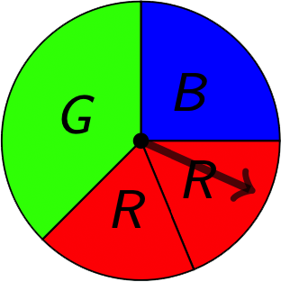
We’ll also use a running example with a colour spinner:
Sample Space
The Sample Space denoted \(\Omega\) is the set of all possible outcomes, or states that a random system could be in.
In the example, the most obvious answer to what the sample space is would be:
\[\Omega = \{ B, G, R \} \]
If you wanted to distinguish between the left red and the right red, you could list the sample space to be:
\[\Omega = \{B, G, R_\mbox{left}, R_\mbox{right}\} \]
If we wanted to concentrate on the angle of the spinner arrow, the sample space would be:
\[\Omega = [0, 2\pi) \]
Further still, if you consider the direction (clockwise, or anti-clockwise) in which you flick the arrow and with some strength so that it could go around the revolution multiple times:
\[\Omega = (-\infty, \infty) = \mathbb{R}\]
Events
An Event is a subset of the sample space, of which we can measure its probability.
Usually, we can describe an event with words, such as “the spinner does not land on green.” In the running example, this would be the subset \(\{B, R\}\).
In the definition of an event, the latter part “… of which we can measure its probability” – is of greater importance in the study of Measure Theory, so for the sake of this post we’ll assume that every subset in the sample space has a probability – in general this is not always true.
The set of all possible events is called the Event Space, denoted by \(\mathcal{A}\). Some things to note about the event space are the following:
- complements of events are also events.
For example, \(\{B, R\}\) is in \(\mathcal{A}\), i.e. it is an event, implies that the complement subset \(\{G\}\) is also in \(\mathcal{A}\), so it is also an event. - countable unions and intersections of events are also events.
- the empty set \(\emptyset\) (called an impossible event) and the sample space \(\Omega\) (called a certain event) are events.
In the running example, the event space turns out to be the power set, the set of all subsets, of \(\Omega\). So:
\[\mathcal{A} = \{ \emptyset, \{B\}, \{G\}, \{R\}, \{B, G\}, \{B, R\}, \{G, R\}, \{B, G, R\}\} \]
Probability of Events
The function \(P: \mathcal{A} \rightarrow [0,1]\) is the probability measure of an event.
This function maps every event in the event space to a probability between 0 and 1 inclusive. It also has to obey a few rules:
- \(P(\emptyset) = 0\) – the probability of an impossible event must be \(0\).
- \(P(\Omega) = 1\) – the probability of a certain event must be \(1\).
- for all natural numbers \(n\), \(P\left( A_1 \cup A_2 \cup \ldots \cup A_n \right) = \sum_{k=1}^n P(A_k)\) if each \(A_i\) in the union are pairwise disjoint.
For the spinner example, we can see that:
\[ P(\{B\}) = \frac{1}{4}, P(\{G\}) = \frac{3}{8}, P(\{R\}) = \frac{3}{8}\]
We can use the third property listed above to work out the probability of any other event that is the union of any one of the sets listed above. For example: \[P(\{B, R\}) = P(\{B\} \cup \{R\}) = P(\{B\}) + P(\{R\}) = \frac{1}{4} + \frac{3}{8} = \frac{5}{8}\]
Random Variables
With all the concepts of probability covered, we can finally turn our attention to random variables. So what is a random variable?
A Random Variable \(X\) is a function:
\[ X: \Omega \rightarrow \mathbb{R} \]
The domain of a random variable is the sample space and the co-domain is the set of real numbers. The random variable is called “discrete” if and only if the range of the random variable is countable. The random variable is called “continuous” if and only if the range of the random variable is uncountable.
Remember from the Syllabus, it states that a random variable “describes some aspect in a population”. The function definition of the random variable achieves this by assigning to each outcome in the sample space, a real number that represents an aspect that it possesses.
In the running example, let’s say that the spinner generates income for a player, and landing on Green or Red generates $4 and landing on Blue generates $1.
We can define a discrete random variable \(X\) that represents the amount of money generated when flicking the spinner as shown below:
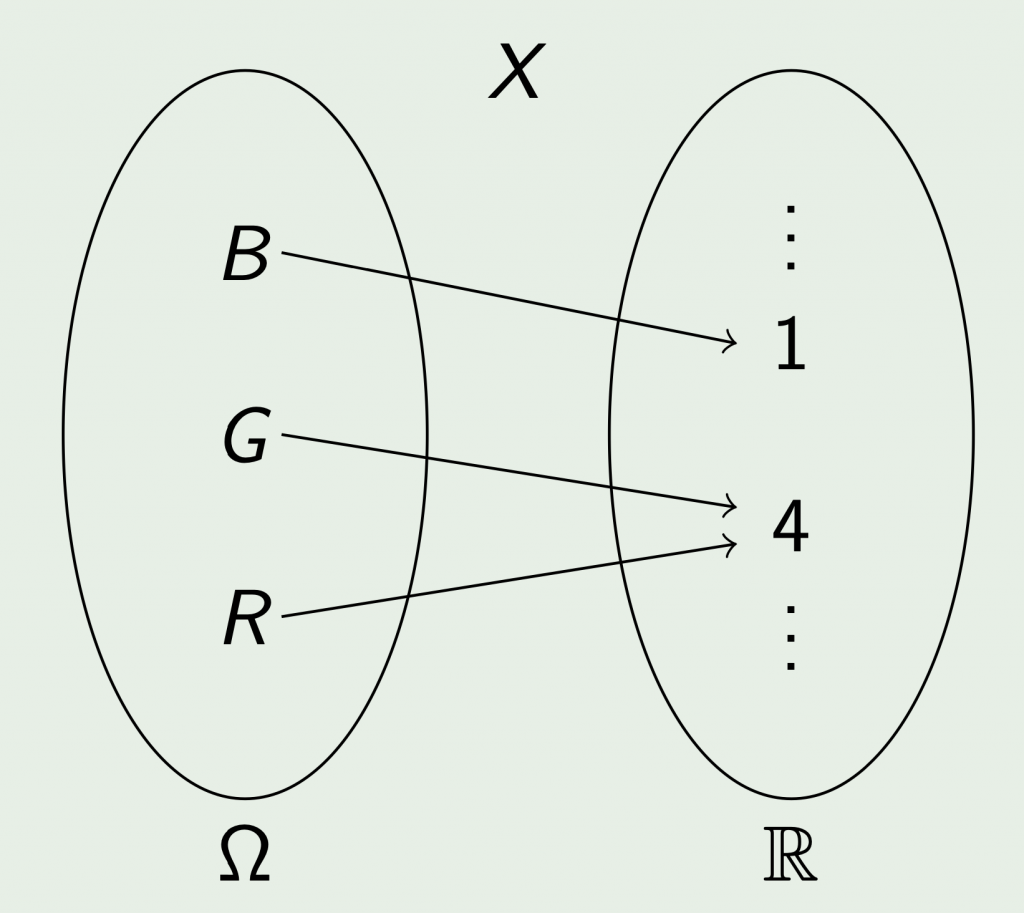
In this function: \[X(B) = 1, X(G) = 4, X(R) = 4\]
Note that in general, the co-domain of a random variable can be any set where measurement is defined, for example: the number plane where the measure of its subsets is the area, 3D space where the measure of its subsets is the volume, and many other sets. For most purposes, it is sufficient to use the real numbers where the subsets of interest are intervals.
Probability of Random Variables
Random Variable Event Notation
Before we can find the probability of random variables, we need to understand one more piece of notation. What does it mean when we write \((X = 4)\)? or \((X<2)\)? or \((-2 < X \leq \pi)\)?
For a subset \(S \subseteq \mathbb{R}\), the notation \(X \in S\) is taken to mean the inverse relation of \(X\) applied to \(S\), i.e.
\[ X \in S = \{ \omega \in \Omega | X(\omega) \in S\} \]
We don’t usually see it written like this with set membership symbols, but instead we see equality and inequality symbols, for example:
\[ (X = 4) = \{ \omega \in \Omega | X(\omega) = 4\}\]
In the running example with the random variable set up, we can see that \((X = 4) = \{G, R\}\) and \((X =1) = \{B\}\).
This notation therefore represents events; recall that they are subsets of the sample space of which we are interested in measuring the probability.
Probability of Random Variables
Now, we can apply the probability measure we had defined on the sample space from before to these events!
We’ll dive straight into the running example:
\[P(X=4) = P(\{G, R\}) = P(\{G\}) + P(\{R\}) = \frac{3}{8} + \frac{3}{8} = \frac{3}{4}\]
We see that the probability of random variables depends on the probability structure of the sample space, and we can actually construct a new function called a Probability Distribution Function \(X_*P: \mathbb{R} \rightarrow [0,1]\) that measures the probability of the random variable.
Note that the HSC notates the probability distribution function as \(f\), and also the probability density function (which we will discuss soon) as \(f\) which isn’t exactly helpful for the sake of the explanation at hand here. Hence, I will opt to use the mathematician Kolmogorov’s notation of \(X_*P\) instead.
This phenomenon where we transferred the probability structure of the event space into the set of real numbers is called a pushforward. This effectively allows us to shortcut going back to the event space to work out the probabilities of the random variable.
In the running example of the spinner, the random variable we’ve defined has a finite range, so we can just tabulate the probability distribution function as below:
| \(x\) | 1 | 4 | else |
| \(P(X=x)\) | \(\frac{1}{4}\) | \(\frac{3}{4}\) | \(0\) |
What About Continuous Random Variables?
In the examples above, we’ve only examined discrete random variables so far. How do we transfer these concepts to a continuous random variable? We can no longer just tabulate the probabilities of each possible event as there are an (uncountably) infinite number of them.
Let’s firstly recap the previous items so far:
- the Sample Space \(\Omega\) contains all possible outcomes.
- subsets of the sample space that we can find the probability of are called Events.
- the set of all events is called an Event Space \(\mathcal{A}\)
- there is a probability measure function \(P: \mathcal{A} \rightarrow [0,1]\).
- the random variable \(X: \Omega \rightarrow \mathbb{R}\) has a pushforward probability distribution function \(X_*P: \mathbb{R} \rightarrow [0,1]\) that measures the probability of the random variable.
Sometimes it’s not obvious how we can construct the pushforward from \(P\), but what we can do instead is compare the rate of change, aka the derivative, of \(X_*P\) with respect to another way we measure the size of subsets in \(\mathbb{R}\).
In developing our theory of integral calculus, we already do this when we partition the \(x\)-axis into smaller width intervals on which we construct rectangles on top of them: in this construction, the size of an interval, say \((a,b)\), is measured as \(b-a\), which we notate as \(\delta x\). As it approaches an infinitesimal length, we notate the measure of the interval as \(dx\).
The rate of change of \(X_*P\) with respect to the usual way of measuring subsets in \(\mathbb{R}\) as in the paragraph above, is called the probability density function, notated as \(f\):
\[ f(x) = \frac{dX_*P}{dx} \]
The fundamental theorem of calculus then allows us to find an expression for \(X_*P\):
\[ P(a < X < b) = \int_a^b f(x) \; dx = X_*P((a,b)) \]
It’s A Wrap!
With that, we now conclude the more than necessary (for HSC) detailed explanation of what random variables are: functions from a domain of the sample space to the co-domain of real numbers. We also looked at the probability of random variables that depend on the probability of the events in the sample space.
What hasn’t been mentioned in this post are calculations that you can do with random variables such as Expected Value and Variance, and the well-known distributions such as Bernoulli, Binomial and Normal Distributions. I’ll discuss these in another post about probability distributions.
A very clear and concise exposé.
Formally a “continuous random variable” X is a random variable taking values in ℝ whose (cumulative) distribution function,
F(x) := P(X ≤ x),
is a continuous function.
In particular,
X: Ω → ℝ a continuous random variable ⇒ P{ ω ∈ Ω : X(ω) = x} = 0
⇒ ∄ ω ∈ Ω such that P({ω}) = 0 (the probability measure has no “atoms”).
A continuous random variable may admit an underlying probability density function,
f : ℝ → ℝ, for which F(x) = int_{-∞}^x f, but this is not necessarily the case.
Errata: P({ω}) = 0 should be P({ω}) does not equal 0.