This is the final part on a series on ‘What Are Numbers?’. In this part, we discuss the construction of the set of the real numbers.
Polynomial Equations
In the previous parts, we constructed the Integers \(\mathbb{Z}\) from Equivalence Classes on the set \(\mathbb{N}\times\mathbb{N}\) that represent the solutions to equations of the form \(x+b =a\). We then constructed the Rational Numbers \(\mathbb{Q}\) from Equivalence Classes on the set \(\mathbb{Z}\times\mathbb{Z}\) that represent the solutions to equations of the form \(bx = a\).
Can we continue doing this and form the real numbers \(\mathbb{R}\) from the equivalence classes on equations? What would these equations be?
One could go down this path and say that we want to form a set of objects that are the roots of the polynomial equations of the form:
\[ c_nx^n + c_{n-1}x^{n-1} + \ldots + c_1x + c_0 = 0\]
where each \(c_i\in\mathbb{Q}\) and \(n \in\mathbb{N}\).
This kind of study goes deep into the incredibly rich theory about rings of polynomials and field extensions, and has awesome implications such as proving when a geometric construction with a straight edge and compass is possible (or impossible), or proving that no general degree 5 and above polynomial equation formula exists! (See Galois Theory).
As an example of what this might entail, let’s have a look at the polynomial equation:
\[x^2 + 3x – 6 = 0\]
One can quickly see that this does not factorise over the rational numbers (also known as irreducible in \(\mathbb{Q}\)). In fact, the definition of the word conjugate we use in our maths classrooms from year 9 (learning about surds for the first time) to year 12 (learning about complex numbers) – actually mean the roots of an irreducible polynomial equation.
By applying the quadratic formula to the equation above, we see that the conjugate roots are \(x = \frac{-3 \pm \sqrt{33}}{2}\).
We know for a fact that \(\sqrt{33}\) is not a rational number. So what we can do is just adjoin it onto the set of rational numbers to get:
\[ \mathbb{Q}(\sqrt{33}) = \{a + b \sqrt{33}| a,b\in\mathbb{Q}\}\]
Elements of this set then solve the equation \(x^2 + 3x – 6 = 0\), as well as create other numbers. In the context of vector spaces over the field \(\mathbb{Q}\), we can see that the set \(\{1, \sqrt{33}\}\) form a linearly independent set whose linear combinations span the whole set. We thus have a basis for \(\mathbb{Q}(\sqrt{33})\).
Without going into the details of why as Field extensions are a rich theory in of themselves, in the context of equivalence classes, we’ve created a new set of numbers based off polynomials with rational coefficients with the same remainder when divided by \(x^2 + 3x – 6\), notated as \(\frac{\mathbb{Q}[x]}{<x^2 + 3x – 6>}\).
Naive Next Steps
A naive notion we can suggest is to just do this with every polynomial, and adjoin every single solution to every single rational polynomial in an attempt to construct the real numbers. However, there’s a lot of problems doing this!
- The set of real numbers is uncountably infinite, i.e. cannot be listed/indexed. The set of any field created by adjoining surds onto the set of rational numbers is countable, i.e. can be listed/indexed.
- We can end up adjoining solutions to polynomial equations such as \(x^2 + 1 = 0\). We know that no real roots exist for such an equation and hence adjoining its unreal roots to \(\mathbb{Q}\) to form \(\mathbb{Q}(i)\) where \(i^2 = -1\) actually goes beyond \(\mathbb{R}\). We could attempt to “fix” this by saying let’s not adjoin any unreal roots.
- Here’s my favourite problem we run into with this attempt. There are real numbers that are not the roots to any polynomial equation! These numbers are called transcendental (as opposed to the algebraic real numbers that are roots to a polynomial equation with rational coefficients). Well known examples include \(\pi\) and \(e\). So adjoining all the roots of all irreducible polynomials under the sun won’t even work as there are some numbers we will miss out on!
So How?
In my research, I have read up on three methods on constructing the Real Numbers (namely using Decimal Expansions, Dedekind Cuts or by Equivalence Classes of Cauchy Sequences). I have opted for the third one in this post as it appeals to me most.
In this section, I’ll attempt to set up the following key concepts:
- Cauchy Sequences in \(\mathbb{Q}\).
- Equivalence classes of Cauchy Sequences.
There’s Sequences, Then There Are Cauchy Sequences
The concept of sequences is covered in the HSC syllabus in Year 12, and oddly under the topic of Financial Mathematics. Sequences are ubiquitous in all of Mathematics, as their behaviours give a lot of insight about the structure of the objects they contain. To shove it into the Financial Mathematics topic seems almost disrespectful or ill-guided in my opinion, but I digress at this point so let’s draw our attention back to the task at hand.
Sequences
A sequence is an enumerated collection of objects, where order matters and repetition is allowed. The notation we use for the nth object in a sequence is \(x_n\).
For example, the sequence of square numbers \(1,4,9,16,25,\ldots\) can be written as \(x_1 = 1\), \(x_2=4\), etc. A general formula can be written down too: \(x_n = n^2\). We can also represent this sequence by writing \(\{n^2\}_{n=1}^\infty\) – note that not all sequences may have a formula, such as the sequence whose nth term is the nth digit of \(\pi\).
Limits
The limit of a sequence is the value that a sequence approaches as \(n\) gets arbitrarily large. We notate this as \(\lim_{n\rightarrow \infty} x_n = x\), or just \(x_n \rightarrow x\). A technical definition of the limit of a sequence is as follows:
\[ \forall \epsilon > 0 \,\exists N\in\mathbb{N} \mbox{ such that } \forall n > N, |x_n – x|<\epsilon \]
This is saying that a sequence has a limit if there is a certain point, say \(n=N\), where all the \(x_{N+1}, x_{N+2}, \ldots \) are within an arbitrary \(\epsilon\) distance away from \(x\).
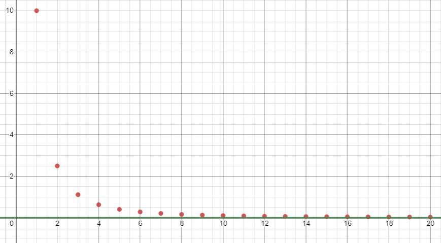
For example, the sequence \(x_n = \frac{10}{n^2}\) has the limit \(x_n\rightarrow 0\).
Cauchy Sequences
A Cauchy sequence is a sequence whose terms get arbitrarily close to one another as the sequence progresses. The definition of this is:
\[ \forall \epsilon > 0\, \exists N\in\mathbb{N} \mbox{ such that }\forall m,n>N\, |x_m – x_n| < \epsilon\]
For example:
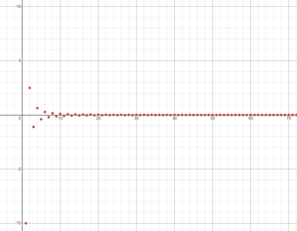
- \(x_n = \frac{10(-1)^n}{n^2}\) is Cauchy.
Not an example:
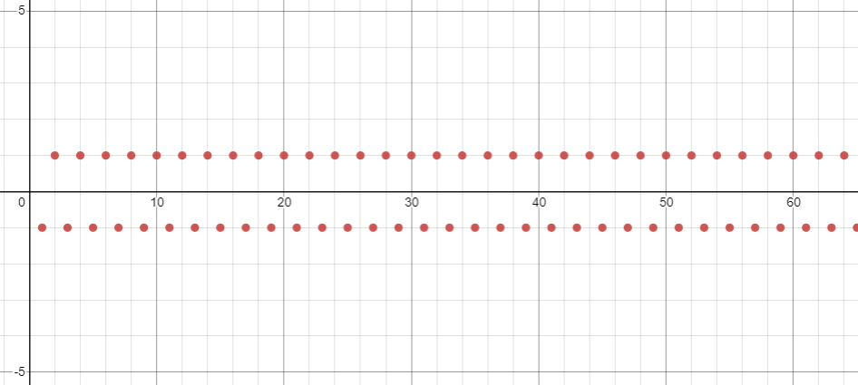
- \(x_n = (-1)^n\) is not Cauchy.
I will denote the set of all Cauchy sequences of rational numbers with the following notation:
\[ S_\mathbb{Q} = \{ \{x_n\}_{n=1}^\infty | x_i \in \mathbb{Q} \mbox{ for } i \in \mathbb{N}\} \]
Limits of Cauchy Sequences
Let’s have a look at the following Cauchy sequence:
\(x_1 = 1\) and \(x_n = x_{n-1} – \frac{x_n^2 -2}{2x_n}\) for \(n > 1\).
Readers may notice that this sequence comes from Newton’s Approximation Method which used to be in the HSC course but has been taken out since the rollout of the new syllabus.
Computing the first few terms we get:
\(1, \frac{3}{2}, \frac{17}{12}, \frac{577}{408}, \frac{665857}{470832},\ldots\)
The decimalisations of these terms (to 9 decimal places as afforded by my CASIO Fx-82AU calculator) are:
\(1, 1.5, 1.416666667, 1.414215686, 1.414213562, \ldots\)
We can see that these terms get progressively closer and closer together, and it is therefore a Cauchy sequence. Note that this informal investigation here is not a proof of the fact, but it’s good enough for our purposes here.
Notice that the decimalisation for \(\sqrt{2}\) to 9 decimal places is \(1.414213562\). We know that \(\sqrt{2}\) is not a rational number, yet the Cauchy sequence of rational numbers we formed earlier is getting closer to it. So while this sequence of rational numbers has a limit, the limit itself is not a rational number!
The key takeaway point is that there are (Cauchy) sequences of rational numbers whose limits are not themselves rational numbers.
Another Cauchy sequence that approaches \(\sqrt{2}\) can be found by the following:
\(x_1 = 50\) and \(x_n = x_{n-1} – \frac{x_n^2 -2}{2x_n}\) for \(n > 1\)
Computing the first few terms and rounding to 9 decimal places we get:
50, 25.02, 12.54996803, 6.354665491, 3.334697441, 1.967226001, 1.491943004, 1.416238394, 1.41421501, 1.414213562, …
Equivalence Classes of Cauchy Sequences
We’ve now identified that there are Cauchy sequences of rational numbers whose limits are not rational. In a sense, they are approaching a “hole” in the set of rational numbers. By forming equivalence classes of all Cauchy sequences with the same limit, we can construct the real numbers by effectively “plugging in the holes”. The reason why this works is left as further investigation into the concept of Metric Spaces and their Completions.
Take a sequence \(\{x_n\}_{n=1}^\infty = x_1, x_2, \ldots\) and another sequence \(\{y_n\}_{n=1}^\infty = y_1, y_2, \ldots\). We can define an equivalence relation by:
\[\{x_n\} \sim \{y_n\} \Leftrightarrow x_n \rightarrow x \mbox{ and } y_n \rightarrow x\]
It’s rather easy to verify that this is an equivalence relation.
Hence, we can form Equivalence Classes on the set of Cauchy sequences of rational numbers to finally get:
\[\mathbb{R} = \frac{S_\mathbb{Q}}{\sim}\]
Each equivalence class in this set can be represented by the limit of these Cauchy sequences. For example:
\(\sqrt{2} = \{(1, \frac{3}{2}, \frac{17}{12}, \frac{577}{408}, \frac{665857}{470832},\ldots), (50, 25.02, 12.54996803, \ldots), \ldots\}\)
And the number \(0\) as an example:
\( 0 = \{(0,0,0,\ldots), (10,5,2.5,1.25,0.625,\ldots), (1, \frac{1}{2}, \frac{1}{3}, \frac{1}{4}, \ldots)\}, \ldots \)
Another thing we should check is that this set we have formed obeys the axiom called the Least Upper Bound Axiom, a fundamental property of the Real Numbers. Further reading on this can be found here: https://en.wikipedia.org/wiki/Least-upper-bound_property
And there you have it! This is how the set of Real Numbers are constructed (with equivalent Cauchy sequences)! The other methods of construction are also quite interesting and worth a look too.
Brief Discussion about Complex Numbers
I’ve decided to leave out the discussion on constructing the Complex Numbers as the theory behind it is quite rich, and I’d probably want to dedicate a post about it another day. Essentially, following on from the previous idea in this post about creating equivalence classes of polynomials, \(\mathbb{C} = \frac{\mathbb{R}[x]}{<x^2 + 1>}\) where we identify equivalence classes of polynomials with same remainders when divided by \(x^2 + 1\).
In line with what was discussed earlier about adjoining elements to an existing field, this is equivalent to adjoining an element \(i\) where \(i^2 = 1\) to the field \(\mathbb{R}\), i.e. \(\mathbb{C} = \mathbb{R}(i)\).
This forms a vector space over \(\mathbb{R}\) with the basis \(\{1, i\}\), so we can think of \(\mathbb{C}\) as equivalent to \(\mathbb{R}^2\), the number plane.
When we think of complex numbers as ordered pairs, their addition and multiplication operations are given by:
\[(a,b) + (c,d) = (a+c, b+d)\]
\[(a,b) \times (c,d) = (ac – bd, ad + bc)\]